Want to know the impact of changing one cell in your spreadsheet on the rest of your data? Want to create interactive scenarios but don’t have time to learn scenarios or programming?
Create an interactive spreadsheet with simple conditional formatting and watch cells change colours when you change a target value.
Video: No programming: Create an interactive spreadsheet with conditional formatting
Apply conditional formatting to a range of cells
- Select a range of cells on the spreadsheet (C6:F16 in this example).


- From the Format menu, click Conditional Formatting.
- Use the Conditional Formatting dialog to specify the criteria to apply, making sure to use cell references rather than fixed values. Then click the Format button and choose how you want the cells which meet the criteria to be formatted (in this example, they appear with a plum-coloured background and white text if their value is greater than the value in cell C2).


Change the target value and be amazed at how values in your table change colours when they meet the target. Or let your boss or you client be amazed at how you brightened their day with an easy to grasp spreadsheet model.